SEML31
Assignment Extension: Chord Recognition
Group TN01 - Team SEML31
Dataset: Reference Annotations: The Beatles
Colab Notebook: Chord_Recognition.ipynb - Colab
Introduction
This project addresses the problem of chord sequence recognition in music audio using a Hidden Markov Model (HMM).
Applications:
- Musicians can play songs by following the chord progression without full score knowledge.
- AI music generation systems can use chord sequences to synthesize music automatically.
We begin with a brief review of the basic music theory concepts.
Basic Music Theory
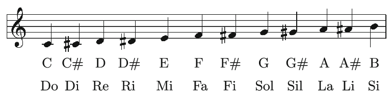
Pitch
In the Western music system, one octave contains 12 notes, with A4 = 440 Hz as the standard tuning reference.
The pitch of all other notes is calculated relative to this reference.
Fundamental Chords
Among various chord types, the two most common are:
- Major chords
- Minor chords
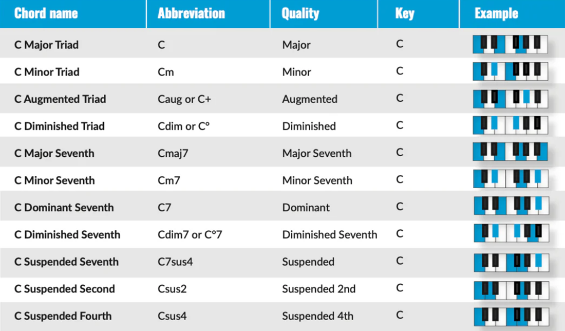
Complex chords occur less frequently. Therefore, in this project, all uncommon chords are converted to either major or minor before training the model.
Each of the 12 notes can serve as the root of one major and one minor chord → 24 states.
An additional state N is added to represent silent sections (no chord).
Dataset
The dataset consists of 50 songs by The Beatles, each including:
- Audio file in MP3 format
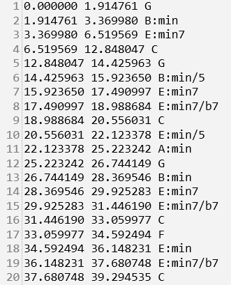
- Annotation file (
.lab) containing chord labels with timing:
start_time end_time chord_label
Each song is randomly segmented into 8 sections to enable the model to learn intermediate musical segments.
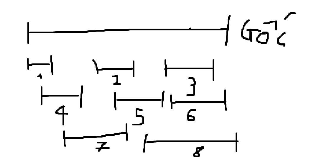
Corresponding .lab files are generated for each audio segment.
Exploratory Data Analysis (EDA)
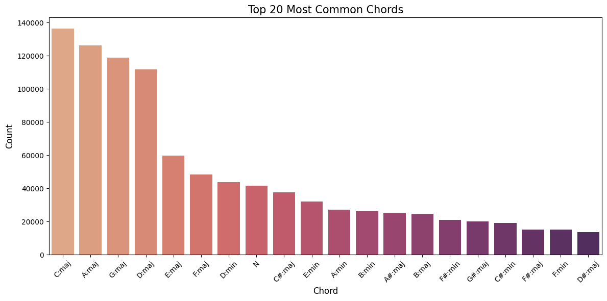
Most Frequent Chords
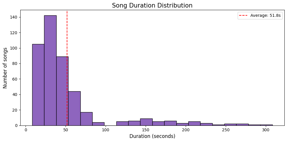
Audio segment statistics:
- Number of segments analyzed: 450
- Average duration: 51.78 seconds
- Shortest duration: 8.24 seconds
- Longest duration: 308.30 seconds
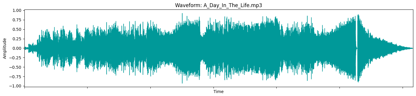
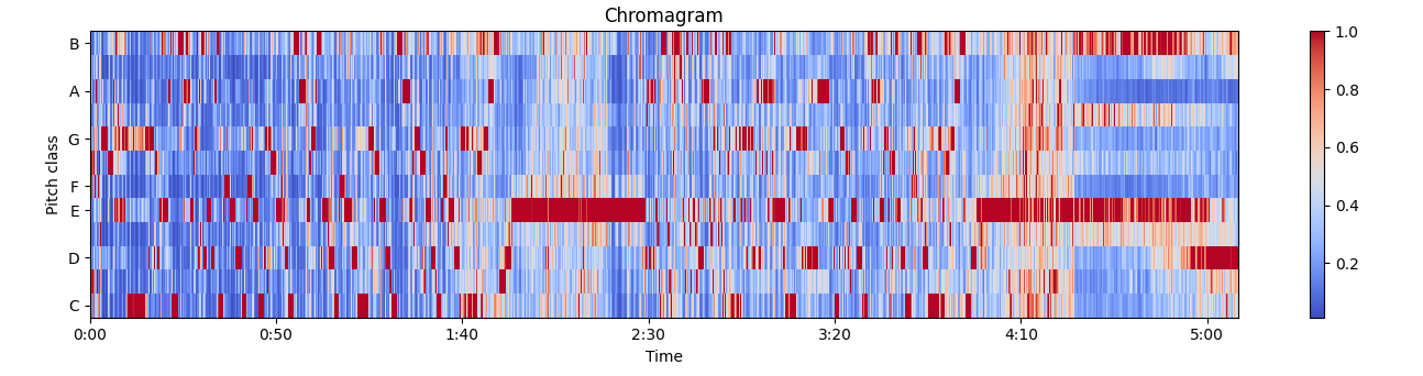
Visualization
Example: A_Day_In_The_Life.mp3
Feature Extraction
The feature extraction pipeline uses Librosa library with a sample rate of 22050 Hz and hop length of 512 samples .
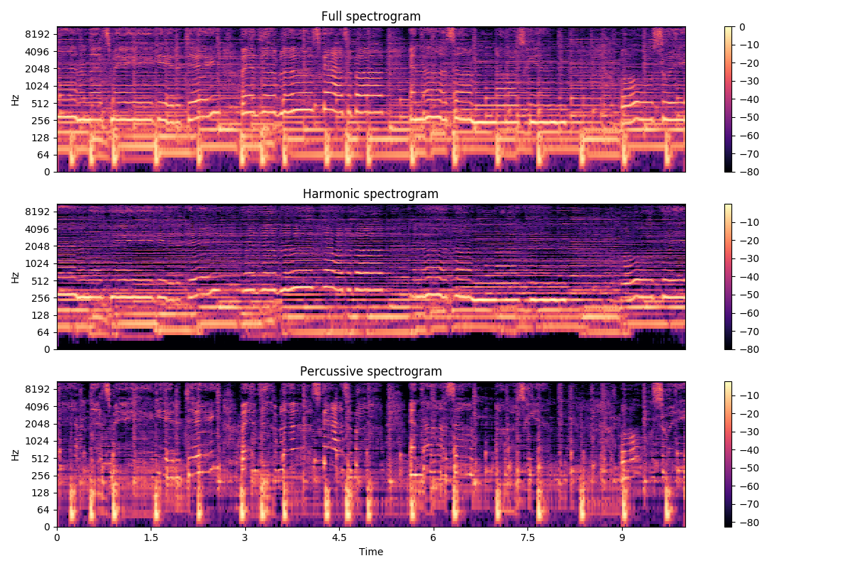
1. HPSS (Harmonic/Percussive Source Separation)
Separates harmonic and percussive components to remove drum signals, which do not contribute to chord recognition.
2. Audio Features
2.1. Chroma CQT (12 dimensions)
Measures the energy of the 12 pitch classes in each time frame using Constant-Q Transform with 48 bins per octave for higher frequency resolution.
2.2. Tonnetz (6 dimensions)
Tonal Centroid Features representing harmonic relationships between notes in tonal space. Captures tonal context beyond simple pitch content.
2.3. Spectral Contrast (7 dimensions)
Measures the difference in amplitude between peaks and valleys in the spectrum across 6 frequency bands plus the mean. Captures timbral texture and harmonic richness.
2.4. Delta Features (25 dimensions each)
- Delta (1st order): Captures temporal dynamics - how features change over time
- Delta-Delta (2nd order): Captures acceleration of feature changes
3. Additional Processing
3.1. Median Filtering
Applied to all feature matrices (Chroma, Tonnetz, Spectral Contrast) using a 1D median filter with window size of 3 along the time axis. This technique removes outliers and smooths temporal variations while preserving sharp transitions between chords.
3.2. L2 Normalization
Each feature vector is normalized to unit L2 norm (Euclidean length = 1). This ensures that features are scale-invariant across different audio volume levels, making the model robust to loudness variations in the input audio.
Total: 12 + 6 + 7 + 25 + 25 = 75 dimensions
HMM Model
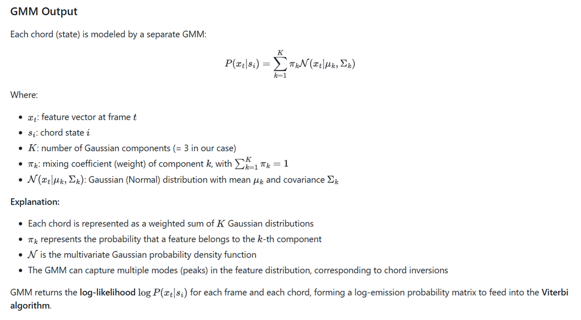
Gaussian Mixture Model (GMM) for Emission Probabilities
Why GMM?
In traditional HMMs, the emission matrix B is designed for discrete observations. However, audio features extracted (Chroma, Tonnetz) are continuous features.
Therefore, we use Gaussian Mixture Model (GMM) to model the probability distribution of features for each chord, replacing the discrete emission matrix.
Results
Overall Accuracy: 42.77%
Confusion Matrix
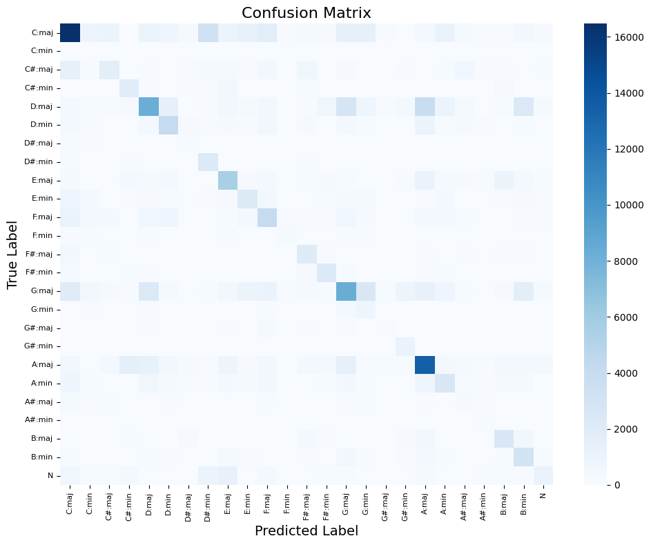
Discussion
Although the dataset was augmented, the overall accuracy remains moderate.
The chords most frequently recognized correctly are Cmaj, Dmaj, Amaj, Gmaj, which also correspond to the most common chords identified in the EDA.
Future Improvements
Future work will employ wavelet-based feature extraction to better capture the characteristics of music