SEML31

Assignment 1: Tabular Data

Group TN01 - Team SEML31

Colab Notebook:

The problem

• Dataset: Rain in Australia
  • Tabular dataset type.
  • 10 years of daily weather observations from numerous Australian weather stations.
• Given the data of the current day, we need to predict whether it would rain the following day.
• Binary classification model: For each sample in the dataset (a row in the table)
  • Input: The features of a sample.
  • Output: The prediction of that sample (rain or no rain tomorrow).

Exploratory Data Analysis (EDA)

• The dataset table has shape (145460, 23). There are 145000+ samples, and 23 columns including the label RainTomorrow.
  • Numerical columns: ['MinTemp', 'MaxTemp', 'Rainfall', 'Evaporation', 'Sunshine', 'WindGustSpeed', 'WindSpeed9am', 'WindSpeed3pm', 'Humidity9am', 'Humidity3pm', 'Pressure9am', 'Pressure3pm', 'Cloud9am', 'Cloud3pm', 'Temp9am', 'Temp3pm']
  • Categorical columns: ['Date', 'Location', 'WindGustDir', 'WindDir9am', 'WindDir3pm', 'RainToday', 'RainTomorrow']
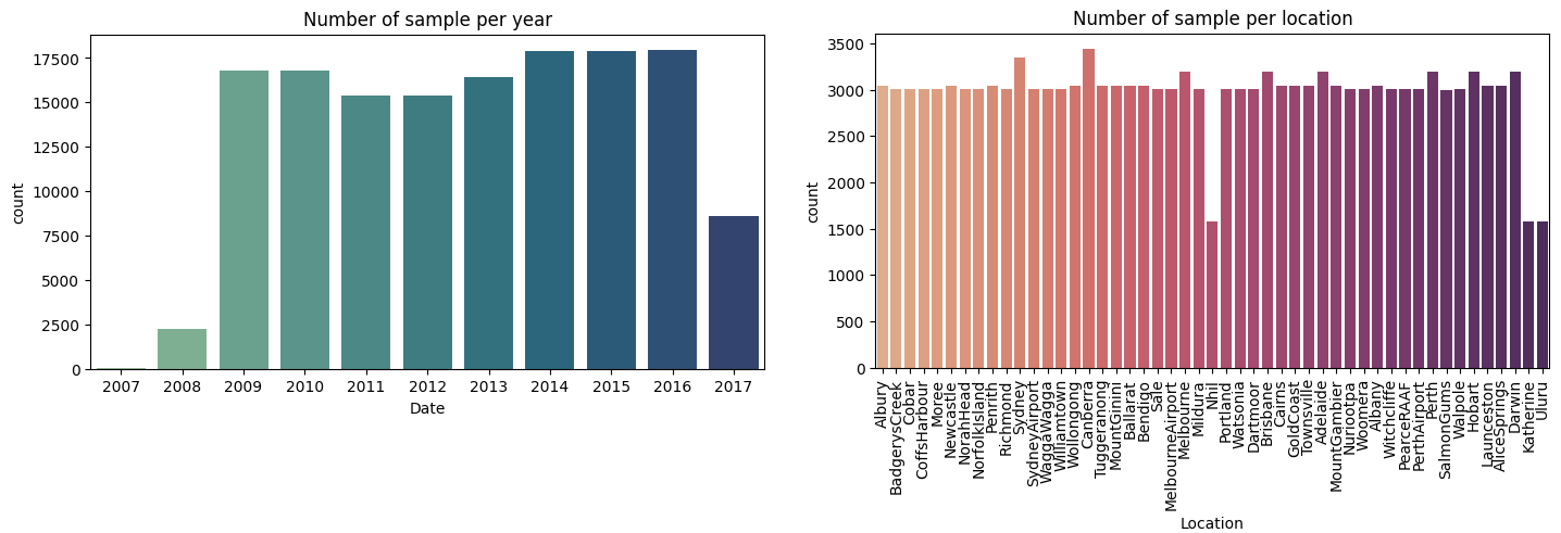
• The number of sample stay consistantly high from 2009 to 2016, with consistant sample all around Australia.
  
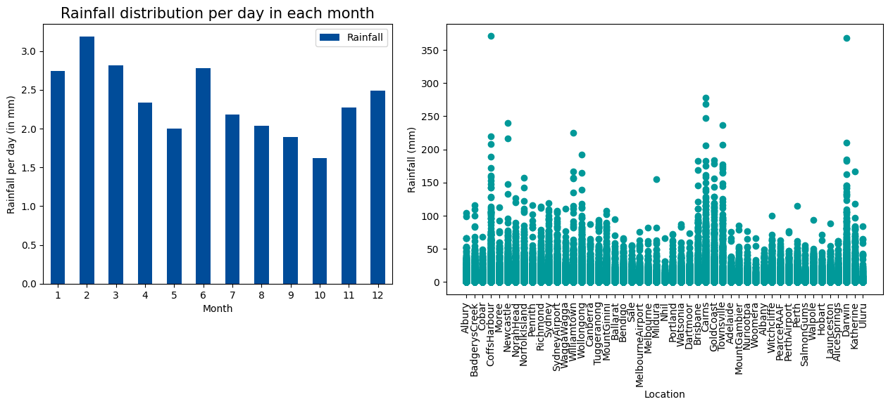
• Rainfall can varied by month. According to www.australia.com, the rainy season in North Australia falls between November and April. Some location may rain more than the others.
  
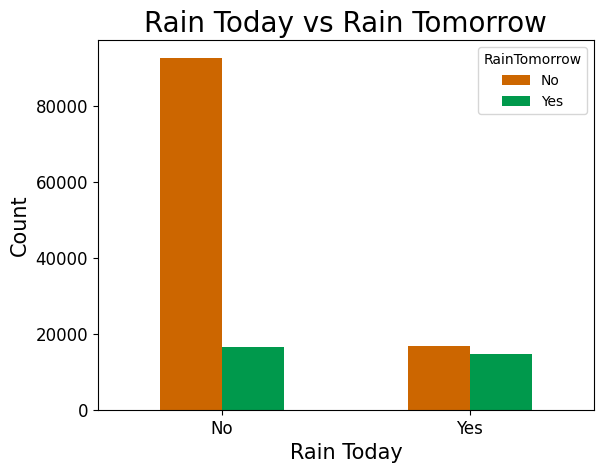
• If it doesn’t rain today, then it’s likely that it won’t rain tomorrow.
  
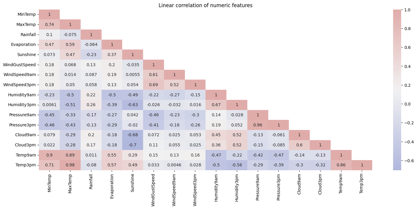
• The correlation matrix shows that temperature, evaporation, humidity, and pressure are quite correlated. Among the various numerical features, humidity has the most correlation with rainfall.
  

Preprocess

The preprocess pipeline has the following configurations:

• up_sampling: If True, upsample the “No” label samples to be equal to the number of “Yes” label samples. If False, downsamlpe the “Yes” label.
• drop_outlier: If True, drop the samples that contain outlier features. For each numerical feature, the outlier range is determined to be from the first quartile to the third quartile.
• fill_na: Replace the NaN values with the median or the mean of the column.
• cat_encode: Encoding ordinal or onehot for categorical columns.
• scale: Can be norm or minmax scaler
• pca_variance: Float value between 0 and 1.

The preprocess pipeline also splits the Date column into day, month, year; drop the rows where the label RainTomorrow is NaN; and splits the dataset into train and test sets.

Training result

The following preprocess configuration is chosen for training. We have a total of 8 preprocessing combinations.

1. fill_na: median, mean
2. cat_encode: ordinal, onehot
3. pca_variance: 0.9, None

We used 5 machine learning models, trained using Scikit-learn and PyTorch with the following configurations:

1. K-Nearest Neighbors, n_neighbors: 5, 11
2. Logistic Regression, penalty: l2, None
3. Random Forests, n_estimators: 50, 100
4. XGBoost, learning_rate: 0.1, 0.3
5. MLP (pytorch), num_hidden: 2, 3

In total, with 10 model configurations, each trained with 8 preprocessed configurations, we get a total of 80 models. Here we only show the result table of XGBoost, with the highest f1-score model highlighted (click here to see the rest):

model_config	fill_na	encode	pca	accuracy	precision	recall	f1
0.1	median	ordinal	0.9	0.818974	0.818315	0.78145	0.799458
0.1	median	ordinal	None	0.840999	0.851672	0.79392	0.821783
0.1	median	onehot	0.9	0.819261	0.816677	0.784723	0.800382
0.1	median	onehot	None	0.839919	0.851417	0.791426	0.820326
0.1	mean	ordinal	0.9	0.819333	0.818256	0.782541	0.8
0.1	mean	ordinal	None	0.846757	0.863097	0.794076	0.827149
0.1	mean	onehot	0.9	0.819405	0.817045	0.784567	0.800477
0.1	mean	onehot	None	0.845966	0.864574	0.790179	0.825705
0.3	median	ordinal	0.9	0.829986	0.829138	0.795791	0.812122
0.3	median	ordinal	None	0.846469	0.851907	0.80795	0.829346
0.3	median	onehot	0.9	0.826315	0.825049	0.791738	0.80805
0.3	median	onehot	None	0.849061	0.853934	0.812003	0.832441
0.3	mean	ordinal	0.9	0.831138	0.829154	0.798909	0.81375
0.3	mean	ordinal	None	0.850932	0.860438	0.808262	0.833534
0.3	mean	onehot	0.9	0.830922	0.830569	0.796259	0.813052
0.3	mean	onehot	None	0.850788	0.861352	0.806703	0.833132

Comparing the highest f1 score configurations in each type of model against each other:

classifier	model_config	fill_na	encode	pca	accuracy	precision	recall	f1
K-Nearest Neighbors	11	mean	onehot	None	0.814223	0.813645	0.775214	0.793965
Logistic Regression	None	median	onehot	None	0.777442	0.769243	0.739984	0.754330
Random Forest	100	mean	ordinal	None	0.836536	0.845103	0.790959	0.817135
XGBoost	0.3	mean	ordinal	None	0.850932	0.860438	0.808262	0.833534
MLP	2	median	onehot	None	0.815950	0.781770	0.834295	0.807179

Remark

• Among all models with their best configurations, XGBoost is the model with the highest f1-score. This suggests it has good performance in handling tabular data.
• PCA: For the best performing configurations, PCA was not applied (pca=None). This suggests that the original feature space was more effective for these models.
• Encoding: Both ordinal and onehot encoding methods is effective depending on the model.
• Imputation: Both median and mean imputation give good results, this can mean this step doesn’t affect the performance much.